🎯 Create a connected query
Open Power BI Desktop and load a pbix file containing the data you want to connect to.
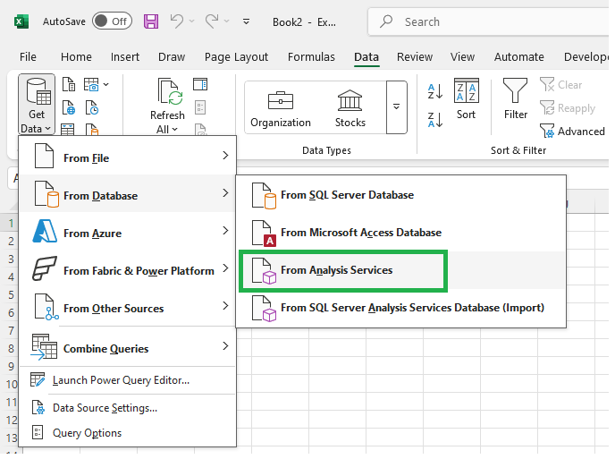
In Excel, click the Connect button in the pbixl tab.
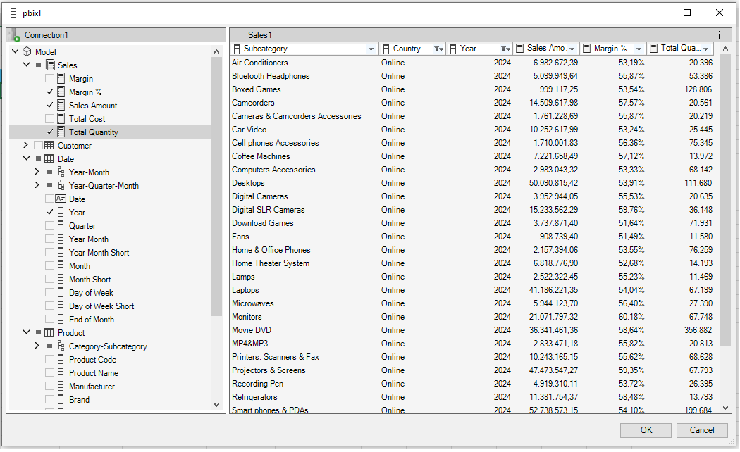
Select a measure and some columns.
click image
Open Power BI Desktop and load a pbix file containing the data you want to connect to.
In Excel, click the Connect button in the pbixl tab.
Select a measure and some columns.
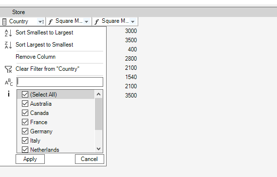
Filtering can be done by selecting elements or by providing a search term.
A search term can be created using the AND and OR operators in conjunction with brackets.
To Return "amounts below 1000 and between 10000 and 20000" would be written as: <1000 or (>=10000 and <=20000)
On date columns, just write 2024 to get all dates in 2024.
Text columns can be filtered using asterisks.
The filter dialog provides an info icon. Click it to see sample search terms.
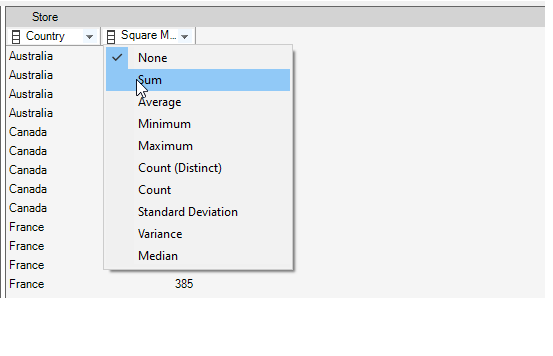
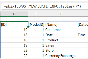
Standard functions like sum(), max(), count() can be applied to columns.
Click on the left symbol of the column to select functions.
In the top right corner is an info button. Click it to inspect the created DAX statement.
Use an Excel dynamic array formula to execute any DAX statement from Power BI Desktop or
Power BI Service and get data into your worksheet.
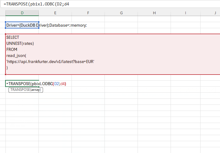
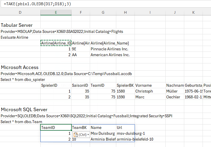
Provide a connection string to connect to any ODBC or OLEDB database.
Use the database engine of your choice to take advantage of its features and query capabilities.
In Excel, click the Connect button in the pbixl tab.
Click the arrow on the OK button and select Pivot Table.
Click OK.
Every time you close and reopen Power BI Desktop, the connection changes.
pbixl tries to reconnect the Excel workbook to the changed PBI Desktop connection.
When reconnecting Excel, please open Power BI first, then the Excel workbook.
Give a Power BI model a unique name by creating a hidden measure in the model.
pbixl = "myContoso"
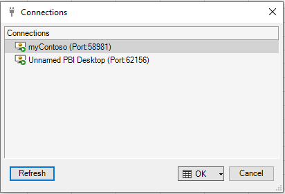
Provide a connection to Power BI Service or a SSAS Tabular model in your workbook.
Get a connected workbook from PBI Service by using the Analyze in Excel feature.
Connect a workbook to SSAS Tabular by using the Get Data feature of Excel.
The connection appears in the Connect dialog of pbixl.